linktree vignette
linktree_vignette.Rmdlinktree
The goal of linktree is to estimate the transmission
assortativity coefficient. More information here.
Installation
pacman::p_load_gh("CyGei/linktree")Understanding the transmission assortativity coefficient
The linktree framework uses transmission chain data to
estimate group transmission assortativity, which
quantifies the tendency of individuals to transmit within their
own group relative to other groups.
It is defined as the relative increase, or decrease, in the probability of within-group transmission compared to what would be expected under random transmission. Random transmission expectations are calculated based on the group’s relative size, defined as proportion of the total susceptible population that belongs to the group.
The metric characterises transmission patterns, reflecting both contact patterns and group-specific differences in susceptibility or infectiousness.
Gamma
ranges from to , where:
represents homogeneous (random) transmission:
Individuals in group A are equally likely to transmit in A as in other groups.>1 indicates assortative transmission:
Individuals in group A are more likely to transmit in A than in other groups.indicates disassortative transmission:
Individuals in group A are less likely to transmit in A than in other groups.
For example, if , individuals in group A are twice more likely to transmit within group A compared to other groups. Conversely, if , individuals in group A are half as likely to transmit within group A compared to other groups.
Delta
To simplify interpretation, we introduce a rescaled parameter , ranging between (fully disassortative) and (fully assortative), with 0 indicating homogeneous patterns.
We can visualise the relationship between and :
delta <- seq(-1, 1, 0.1)
gamma <- delta2gamma(delta)
plot(gamma, delta, type = "l")
points(1, 0, col = "red", pch = 16)  # Homogeneous
Estimation
get_gamma and get_delta estimate
and
from a transmission tree. It requires the following inputs:
from: a vector of infector’s group (e.g. age group, sex, vaccination status, etc.).to: a vector of infectee’s group.f: a named vector of the groups’ sizes or relative sizes (i.e. proportion of the population in each group).
Example
Data
We can simulate an outbreak with multiple groups using the o2groups
package and then use linktree to estimate the assortativity
coefficients from the transmission tree. Below is a pre-loaded simulated
transmission tree, see ?sim_tree for more details.
#?sim_tree
true_gammas <- c(HCW = 2, patient = 1/1.25)
sizes <- c(HCW = 100, patient = 350)
# data(sim_tree)
sim_tree <- read.csv("https://raw.githubusercontent.com/CyGei/linktree/refs/heads/main/vignettes/sim_tree.csv")
head(sim_tree)
#>     group     id source source_group date_infection date_onset
#> 1     HCW HmPsw2   <NA>         <NA>              0         12
#> 2 patient WtYSxS   <NA>         <NA>              0         12
#> 3 patient gZ6tF2   <NA>         <NA>              0          3
#> 4 patient Kxtgdz   <NA>         <NA>              0          1
#> 5 patient aH9xtg gZ6tF2      patient              1          5
#> 6     HCW DJE8PP gZ6tF2      patient              2          5
Visualise the transmission tree
remotes::install_github('reconhub/epicontacts@timeline')
#>
#> ── R CMD build ─────────────────────────────────────────────────────────────────
#> * checking for file ‘/tmp/Rtmp5IGOmW/remotes200245a29076/reconhub-epicontacts-417f972/DESCRIPTION’ ... OK
#> * preparing ‘epicontacts’:
#> * checking DESCRIPTION meta-information ... OK
#> * checking for LF line-endings in source and make files and shell scripts
#> * checking for empty or unneeded directories
#> Removed empty directory ‘epicontacts/figs’
#> * building ‘epicontacts_1.2.0.tar.gz’
library(epicontacts)
library(visNetwork)

x <- epicontacts::make_epicontacts(
  linelist = sim_tree[, c("group", "id", "date_infection", "date_onset")],
  contacts = sim_tree[, c("source", "id", "source_group", "group")],
  id = "id",
  from = "source",
  to = "id",
  directed = TRUE
)

plot(x,
    method = "visNetwork",
    x_axis = "date_infection",
    label = FALSE,
    node_color = "group",
    node_shape = "group",
    shapes = c(patient = "bed", HCW = "user-md"),
    edge_color = "source_group",
    edge_width = 1,
    node_size = 20,
    col_pal = epicontacts::spectral,
    edge_col_pal = epicontacts::spectral
  ) %>%
  visNetwork::visEdges(shadow = TRUE,
                       arrows = list(to = list(enabled = TRUE, scaleFactor = 0.1)))
Estimate the transmission assortativity coefficient
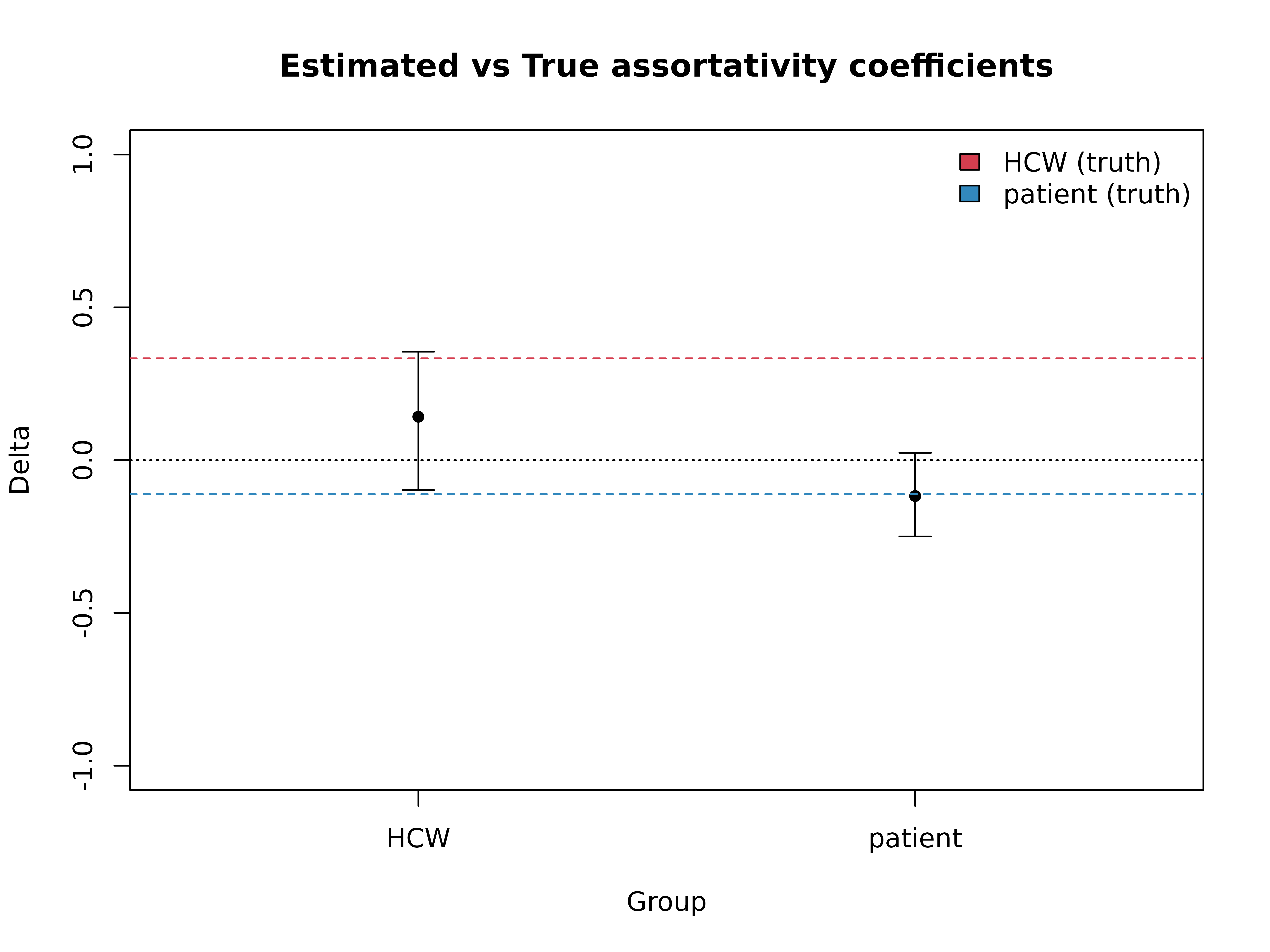
Our published paper provides guidelines as to when and under which circumstances we can reliably infer group transmission assortativity. Notably, we should analyse transmission chains up to the group’s epidemic peak to avoid the saturation effect, and we should have at least ~30 cases in the group.
est_delta <- get_delta(
  from = sim_tree$source_group,
  to = sim_tree$group,
  f = sizes,
)
true_deltas <- gamma2delta(true_gammas)

plot(est_delta, main = "Estimated vs True assortativity coefficients")
abline(h = true_deltas, col = c("#d53e4f", "#3288bd"), lty = 2)
legend("topright", legend = c("HCW (truth)", "patient (truth)"), fill = c("#d53e4f", "#3288bd"), bty = "n")