Extended analyses
extended_analyses.RmdReproduction number
We can estimate the case reproductive number
(),
i.e. the number of secondary infections generated by each case,
with the get_Ri function:
out_id <- identify(out, linelist$name)

# A matrix of R values
# Columns refer to the case ID
# Rows refer to the MCMC iteration
Ri_mat <- get_Ri(out_id)
You can plot the offspring distribution:
Ri_mat %>%
  mutate(step = row_number()) %>%
  pivot_longer(-step, names_to = "name", values_to = "Ri") %>%
  group_by(step, Ri) %>%
  summarise(n = n(), .groups = "drop_last") %>%
  mutate(percent = n / sum(n) * 100) %>%
  ungroup() %>%
  group_by(Ri) %>%
  summarise(
    mean = mean(percent),
    lower = quantile(percent, 0.025),
    upper = quantile(percent, 0.975),
    .groups = "drop"
  ) %>%
  ggplot(aes(x = Ri, y = mean)) +
  geom_segment(aes(x = Ri, xend = Ri, y = 0, yend = mean), colour = "grey60", size = 0.5) +
  geom_point(size = 2) +
  geom_errorbar(aes(ymin = lower, ymax = upper), width = 0.2) +
  labs(x = "Number of secondary infections (Ri)",
       y = "Mean % of cases",
       title = "Posterior offspring distribution with 95% credible intervals")+
  theme_bw()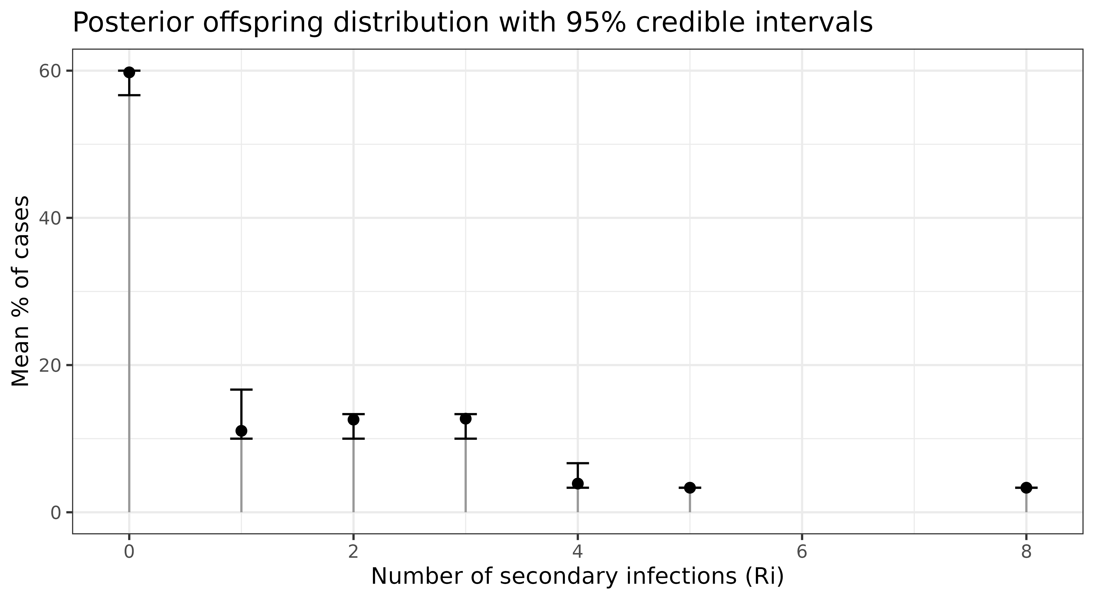
Serial interval
The serial interval (SI) is the time between the onset of symptoms in
an infector-infectee pair. You can compute the SI’s empirical cumulative
density functionusing with get_si() :
trees <- get_trees(out_id, onset = linelist$onset)
si <- get_si(trees, date_suffix = "onset")

si |>
  ggplot(aes(x = x, y = mean))+
  geom_point() +
  geom_ribbon(aes(ymin = lwr, ymax = upr),
              fill = "grey",
              alpha = 0.5) +
  labs(x = "serial interval", y = "Percent")+
  theme_bw()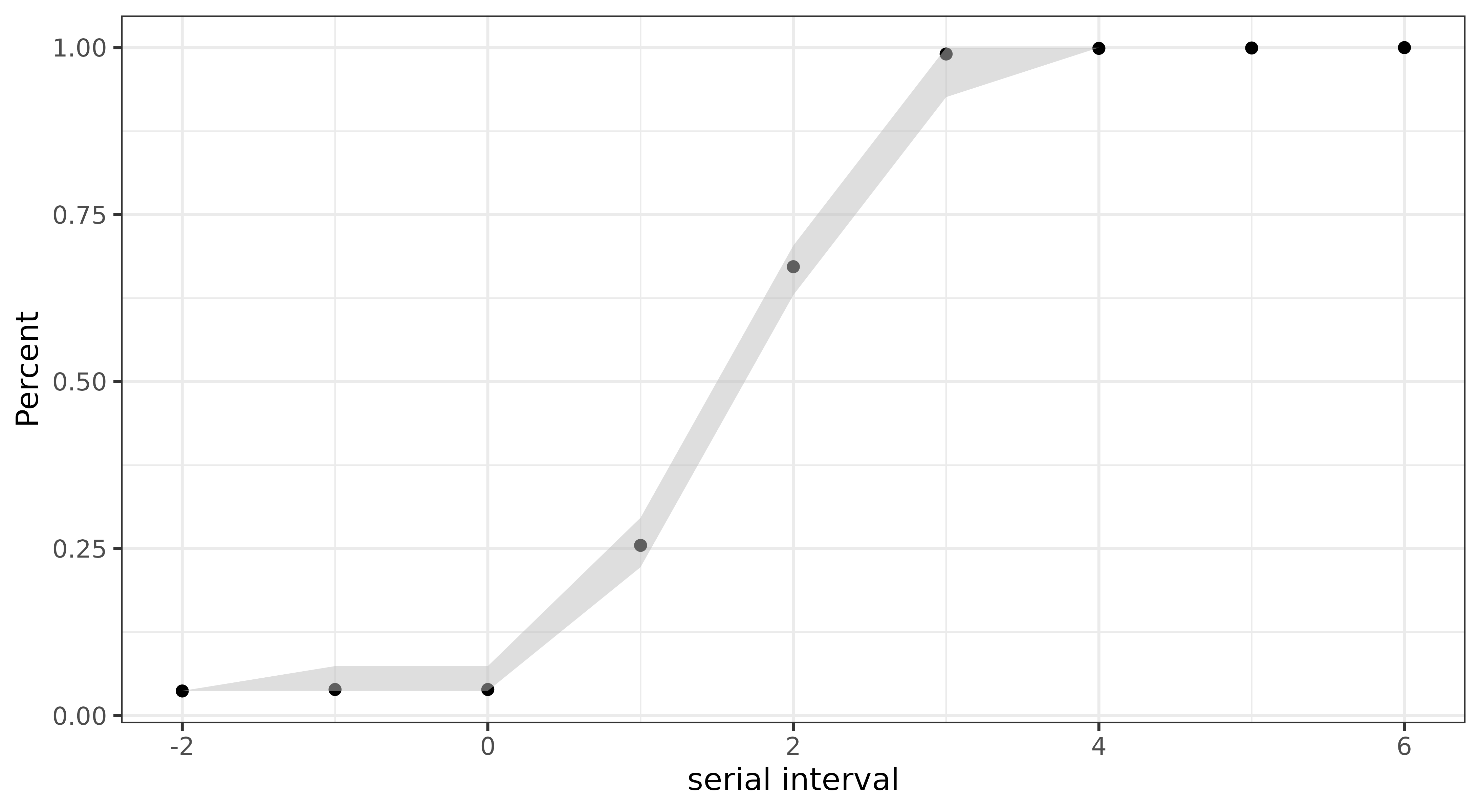
Model convergence
outbreaker2 uses Bayesian inference to account for
uncertainty in who infected whom by sampling multiple plausible
transmission trees from the posterior distribution. Standard MCMC
diagnostics evaluate parameter chains (see
?plot.outbreaker_chains and
?coda::gelman.diag) rather than transmission events
themselves.
mixtree provides a statistical framework for comparing collections of transmission trees (epidemic forests) to assess whether they originate from the same generative process. To evaluate MCMC convergence, mixtree can be used to compare epidemic forests sampled from multiple parallel MCMC chains. If the chains have converged, the resulting epidemic forests should be statistically indistinguishable.
Run multiple chains of outbreaker2
data <- outbreaker_data(dna = fake_outbreak$dna, dates = linelist$onset, ctd = fake_outbreak$ctd, w_dens = fake_outbreak$w)

# Run multiple chains of outbreaker2 in parallel with furrr
library(furrr)
n_chains <- 5
plan(multisession, workers = n_chains) #make sure to set the number of workers to the number of cores on your machine

set.seed(123)
chains <- future_map(1:n_chains, function(i) {
  out <- outbreaker(data = data)
  #brunin
  out[out$step>500, ]
}, .options = furrr_options(seed = TRUE))
Extract trees
We now have 5 epidemic forests, one for each chain.
Chi-squared test
library(mixtree)

set.seed(123)
do.call(what = mixtree::tree_test, args = c(trees, list(
  method = "chisq",
  test_args = list(simulate.p.value = TRUE, B = 999)
)))
#>
#>  Pearson's Chi-squared test with simulated p-value (based on 999
#>  replicates)
#>
#> data:  count data
#> X-squared = 78.327, df = NA, p-value = 1
We used the chi-squared test to test the null hypothesis that the frequency of infector-infectee pairs is the similar between forests. A p-value of 1 indicates similarity between the forests, suggesting convergence. The chi-squared test allows for multiple introductions, unlike PERMANOVA.
PERMANOVA
PERMANOVA only accepts one introduction event, so we need to re-run
outbreaker2 allowing for a single introduction event only. We
can do this by setting the find_import argument to
FALSE.
set.seed(123)
chains <- future_map(1:n_chains, function(i) {
  out <- outbreaker(
    data = data,
    config = outbreaker2::create_config(find_import = FALSE, move_kappa = FALSE)
  )
  #brunin
  out[out$step>500, ]
}, .options = furrr_options(seed = TRUE))

trees <- lapply(chains, function(x) {
  tree_list <- get_trees(x)
  lapply(tree_list, function(tree) {
    # Remove the imported case
    tree[!is.na(tree$from), ]
  })
})

set.seed(123)
do.call(what = mixtree::tree_test, args = c(trees, list(
  method = "permanova",
  test_args = list(permutations = 100)
)))
#> Permutation test for adonis under reduced model
#> Permutation: free
#> Number of permutations: 100
#>
#> (function (formula, data, permutations = 999, method = "bray", sqrt.dist = FALSE, add = FALSE, by = NULL, parallel = getOption("mc.cores"), na.action = na.fail, strata = NULL, ...)
#>           Df SumOfSqs      R2      F Pr(>F)
#> Model      4     3156 0.00493 1.1703 0.2772
#> Residual 945   637030 0.99507
#> Total    949   640185 1.00000
PERMANOVA tests whether the variance in tree topology is similar between forests. A p-value > 0.05 suggests that the topologies of the trees do not differ significantly across the 5 forests, suggesting convergence.
Group transmission patterns
Transmission chains can inform on the patterns of transmission between groups. linktree provides a framework for estimating group transmission assortativity which quantifies the extent to which individuals transmit within their own group compared to others.
This requires knowledge of group sizes or their relative proportions. In our example, say the staff-to-patient ratio in the hospital is 1:3. It is also advised to analyse the transmission chains before saturation (i.e. the epidemic peak).
Estimate the peak date
We’ll estimate the peak date with the incidence2 package.
library(incidence2)
linelist$date_onset <- as.Date(linelist$onset, origin = "2020-01-01")

incid <- incidence2::incidence(linelist,
                               date_index = "date_onset",
                               groups = "group")
peak <- estimate_peak(regroup(incid), progress = FALSE)$observed_peak
peak
#> [1] "2020-01-11"
Mask non-direct transmissions
Group transmission assortativity is estimated from direct
transmissions only. We can use the filter_chain function to
mask non-direct transmissions (i.e. where
kappa>1).
out_direct <- filter_chain(
  out,
  param = "kappa",
  thresh = 1,
  comparator = "==",
  target = "alpha" # keep alpha values where kappa == 1
)

trees <- get_trees(out_direct,
                   group = linelist$group,
                   onset = linelist$date_onset)

# keeps only rows where both onset dates are on or before peak
cut_trees <- lapply(trees, function(tree) {
  tree |> filter(from_onset <= peak, to_onset <= peak)
})
Estimate group transmission assortativity
To run the below you need to install linktree from GitHub.
For a given tree, we can estimate the groups’ transmission assortativity coefficients with:
library(linktree)
# staff-to-patient ratio
ratio <- c("hcw" = 1, "patient" = 3)

max_post <- trees[[which.max(out$post)]]
delta <- linktree::get_delta(from = max_post$from_group, to = max_post$to_group, f = ratio)
plot(delta)
To account for uncertainty in who infected whom, we can compute the
posterior distribution of assortativity coefficients. This is done by
estimating delta for each tree in the posterior sample.
deltas <- lapply(trees, function(x) {
  linktree::get_delta(from = x$from_group, to = x$to_group, f = ratio)
}) |>
  bind_rows(.id = "tree")

ggplot(deltas) +
  geom_density(aes(x = est, fill = group), bw = 0.03, color = "white") +
  scale_x_continuous(limits = c(-1, 1), breaks = seq(-1, 1, 0.2)) +
  scale_fill_manual(values = c("hcw" = "orange", "patient" = "purple")) +
  theme_classic() +
  theme(legend.position = c(0.1, 0.85))
Convert delta to gamma for
interpretatibilty:
gammas <- deltas |>
  group_by(group) |>
  summarise(
    mean = mean(est),
    q025 = quantile(est, 0.025),
    q975 = quantile(est, 0.975)
  ) |>
  mutate(across(.cols = -group, ~ linktree::delta2gamma(.x)))

head(gammas)
Healthcare workers are nearly 5 times more likely to infect other
HCWs whereas patients are 2.6 (1/0.387) times more likely
to infect other HCWs.